Natural Language is how we, humans, exchange ideas and opinions. There are two main mediums for natural language – speech and text.

Listening and reading are effortless for a healthy human, but they’re difficult for a machine learning algorithm. That’s why scientists had to come up with Natural Language Processing (NLP).

You are viewing: How To Convert Glove Vectors To Binary Format

What is Natural Language Processing?

• NLP enables computers to process human language and understand meaning and context, along with the associated sentiment and intent behind it, and eventually, use these insights to create something new.
• NLP combines computational linguistics with statistical Machine Learning and Deep Learning models.

How do we even begin to make words interpretable for computers? That’s what vectorization is for.

What is vectorization?

• Vectorization is jargon for a classic approach of converting input data from its raw format (i.e. text ) into vectors of real numbers which is the format that ML models support. This approach has been there ever since computers were first built, it has worked wonderfully across various domains, and it’s now used in NLP.

• In Machine Learning, vectorization is a step in feature extraction. The idea is to get some distinct features out of the text for the model to train on, by converting text to numerical vectors.

There are plenty of ways to perform vectorization, as we’ll see shortly, ranging from naive binary term occurrence features to advanced context-aware feature representations. Depending on the use-case and the model, any one of them might be able to do the required task.

Let’s learn about some of these techniques and see how we can use them.

Vectorization techniques

1. Bag of Words

Most simple of all the techniques out there. It involves three operations:

• Tokenization

First, the input text is tokenized. A sentence is represented as a list of its constituent words, and it’s done for all the input sentences.

• Vocabulary creation

Of all the obtained tokenized words, only unique words are selected to create the vocabulary and then sorted by alphabetical order.

• Vector creation

Finally, a sparse matrix is created for the input, out of the frequency of vocabulary words. In this sparse matrix, each row is a sentence vector whose length (the columns of the matrix) is equal to the size of the vocabulary.

Let’s work with an example and see how it looks in practice. We’ll be using the Sklearn library for this exercise.

Let’s make the required imports.

from sklearn.feature_extraction.text import CountVectorizer

Consider we have the following list of documents.

sents = [‘coronavirus is a highly infectious disease’, ‘coronavirus affects older people the most’, ‘older people are at high risk due to this disease’]

Let’s create an instance of CountVectorizer.

cv = CountVectorizer()

Now let’s vectorize our input and convert it into a NumPy array for viewing purposes.

X = cv.fit_transform(sents) X = X.toarray()

This is what the vectors look like:

Let’s print the vocabulary to understand why it looks like this.

sorted(cv.vocabulary_.keys())

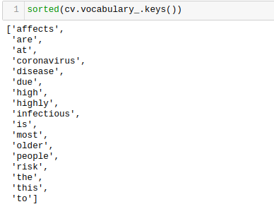
• You can see that every row is the associated vector representation of respective sentences in ‘sents’.
• The length of each vector is equal to the length of vocabulary.
• Every member of the list represents the frequency of the associated word as present in sorted vocabulary.

In the above example, we only considered single words as features as visible in the vocabulary keys, i.e. it’s a unigram representation. This can be tweaked to consider n-gram features.

Let’s say we wanted to consider a bigram representation of our input. It can be achieved by simply changing the default argument while instantiating the CountVectorizer object:

cv = CountVectorizer(ngram_range=(2,2))

In that case, our vectors & vocabulary would look like this.

Thus we can manipulate the features any way we want. In fact, we can also combine unigrams, bigrams, trigrams, and more, to form feature space.

Although we’ve used sklearn to build a Bag of Words model here, it can be implemented in a number of ways, with libraries like Keras, Gensim, and others. You can also write your own implementation of Bag of Words quite easily.

This is a simple, yet effective text encoding technique and can get the job done a number of times.

2. TF-IDF

TF-IDF or Term Frequency-Inverse Document Frequency, is a numerical statistic that’s intended to reflect how important a word is to a document. Although it’s another frequency-based method, it’s not as naive as Bag of Words.

How does TF-IDF improve over Bag of Words?

In Bag of Words, we witnessed how vectorization was just concerned with the frequency of vocabulary words in a given document. As a result, articles, prepositions, and conjunctions which don’t contribute a lot to the meaning get as much importance as, say, adjectives.

TF-IDF helps us to overcome this issue. Words that get repeated too often don’t overpower less frequent but important words.

It has two parts:

1. TF

TF stands for Term Frequency. It can be understood as a normalized frequency score. It is calculated via the following formula:

So one can imagine that this number will always stay ≤ 1, thus we now judge how frequent a word is in the context of all of the words in a document.

1. IDF

IDF stands for Inverse Document Frequency, but before we go into IDF, we must make sense of DF – Document Frequency. It’s given by the following formula:

DF tells us about the proportion of documents that contain a certain word. So what’s IDF?

It’s the reciprocal of the Document Frequency, and the final IDF score comes out of the following formula:

Why inverse the DF?

Just as we discussed above, the intuition behind it is that the more common a word is across all documents, the lesser its importance is for the current document.

A logarithm is taken to dampen the effect of IDF in the final calculation.

The final TF-IDF score comes out to be:

This is how TF-IDF manages to incorporate the significance of a word. The higher the score, the more important that word is.

Let’s get our hands dirty now and see how TF-IDF looks in practice.

Again, we’ll be using the Sklearn library for this exercise, just as we did in the case of Bag of Words.

Making the required imports.

from sklearn.feature_extraction.text import TfidfVectorizer

Again let’s use the same set of documents.

sents = [‘coronavirus is a highly infectious disease’, ‘coronavirus affects older people the most’, ‘older people are at high risk due to this disease’]

Creating an instance of TfidfVectorizer.

tfidf = TfidfVectorizer()

Let’s transform our data now.

transformed = tfidf.fit_transform(sents)

Now let’s see which features are the most important, and which features were useless. For the sake of interpretability, we’ll be using the Pandas library, just to get a better look at scores.

Making the required import:

import pandas as pd

Creating a data frame with feature names, i.e. the words, as indices, and sorted TF-IDF scores as a column:

df = pd.DataFrame(transformed[0].T.todense(), index=tfidf.get_feature_names(), columns=[“TF-IDF”]) df = df.sort_values(‘TF-IDF’, ascending=False)

Since the transformed TFIDF feature matrix comes out as a Scipy Compressed Sparse Row matrix, which can’t be viewed in its raw form, we have converted it into a Numpy array, via todense() operation after taking its transform. Similarly, we get the complete vocabulary of tokenized words via get_feature_names().

This is what comes out of the other end:

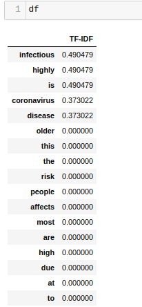
So, according to TF-IDF, the word ‘infectious’ is the most important feature out there, while many words which would have been used for feature building in a naive approach like Bag of Words, simply amount to 0 here. This is what we wanted all along.

A few pointers about TF-IDF:

• The concept of n-grams is applicable here as well, we can combine words in groups of 2,3,4, and so on to build our final set of features.
• Along with n-grams, there are also a number of parameters such as min_df, max_df, max_features, sublinear_tf, etc. to play around with. Carefully tuning these parameters can do wonders for your model’s capabilities.

Despite being so simple, TF-IDF is known to be extensively used in tasks like Information Retrieval to judge which response is the best for a query, especially useful in a chatbot or in Keyword Extraction to determine which word is the most relevant in a document, and thus, you’ll often find yourself banking on the intuitive wisdom of the TF-IDF.

So far, we’ve seen frequency-based methods for encoding text, now it’s time to take a look at more sophisticated methods which changed the world of word embeddings as we know it, and opened new research opportunities in NLP.

3. Word2Vec

This approach was released back in 2013 by Google researchers in this paper, and it took the NLP industry by storm. In a nutshell, this approach uses the power of a simple Neural Network to generate word embeddings.

How does Word2Vec improve over frequency-based methods?

Read more : How Do Boxing Gloves Rip

In Bag of Words and TF-IDF, we saw how every word was treated as an individual entity, and semantics were completely ignored. With the introduction of Word2Vec, the vector representation of words was said to be contextually aware, probably for the first time ever.

Perhaps, one of the most famous examples of Word2Vec is the following expression:

king – man + woman = queen

Since every word is represented as an n-dimensional vector, one can imagine that all of the words are mapped to this n-dimensional space in such a manner that words having similar meanings exist in close proximity to one another in this hyperspace.

There are mainly two ways to implement Word2Vec, let’s take a look at them one by one:

A: Skip-Gram

So the first one is the Skip-Gram method in which we provide a word to our Neural Network and ask it to predict the context. The general idea can be captured with the help of the following image:

Here w[i] is the input word at an ‘i’ location in the sentence, and the output contains two preceding words and two succeeding words with respect to ‘i’.

Technically, it predicts the probabilities of a word being a context word for the given target word. The output probabilities coming out of the network will tell us how likely it is to find each vocabulary word near our input word.

This shallow network comprises an input layer, a single hidden layer, and an output layer, we’ll take a look at that shortly.

However, the interesting part is, we don’t actually use this trained Neural Network. Instead, the goal is just to learn the weights of the hidden layer while predicting the surrounding words correctly. These weights are the word embeddings.

How many neighboring words the network is going to predict is determined by a parameter called “window size”. This window extends in both the directions of the word, i.e. to its left and right.

Let’s say we want to train a skip-gram word2vec model over an input sentence:

“The quick brown fox jumps over the lazy dog”

The following image illustrates the training samples that would generate from this sentence with a window size = 2.

• ‘The’ becomes the first target word and since it’s the first word of the sentence, there are no words to its left, so the window of size 2 only extends to its right resulting in the listed training samples.
• As our target shifts to the next word, the window expands by 1 on left because of the presence of a word on the left of the target.
• Finally, when the target word is somewhere in the middle, training samples get generated as intended.

The Neural Network

Now let’s talk about the network which is going to be trained on the aforementioned training samples.

Intuition

• If you’re aware of what autoencoders are, you’ll find that the idea behind this network is similar to that of an autoencoder.

• You take an extremely large input vector, compress it down to a dense representation in the hidden layer, and then instead of reconstructing the original vector as in the case of autoencoders, you output probabilities associated with every word in the vocabulary.

Input/Output

Now the question arises, how do you input a single target word as a large

Vector?

The answer is One-Hot Encoding.

• Let’s say our vocabulary contains around 10,000 words and our current target word ‘fox’ is present somewhere in between. What we’ll do is, put a 1 in the position corresponding to the word ‘fox’ and 0 everywhere else, so we’ll have a 10,000-dimensional vector with a single 1 as the input.
• Similarly, the output coming out of our network will be a 10,000-dimensional vector as well, containing, for every word in our vocabulary, the probability of it being the context word for our input target word.

Here’s the architecture of how our neural network is going to look like this:

• As it can be seen that input is a 10,000-dimensional vector given our vocabulary size =10,000, containing a 1 corresponding to the position of our target word.
• The output layer consists of 10,000 neurons with the Softmax activation function applied, so as to obtain the respective probabilities against every word in our vocabulary.
• Now the most important part of this network, the hidden layer is a linear layer i.e. there’s no activation function applied there, and the optimized weights of this layer will become the learned word embeddings.
• For example, let’s say we decide to learn word embeddings with the above network. In that case, the hidden layer weight matrix shape will be M x N, where M = vocabulary size (10,000 in our case) and N = hidden layer neurons (300 in our case).
• Once the model gets trained, the final word embedding for our target word will be given by the following calculation:

1×10000 input vector * 10000×300 matrix = 1×300 vector

• 300 hidden layer neurons were used by Google in their trained model, however, this is a hyperparameter and can be tuned accordingly to obtain the best results.

So this is how the skip-gram word2vec model generally works. Time to take a look at it’s competitor.

B. CBOW

CBOW stands for Continuous Bag of Words. In the CBOW approach instead of predicting the context words, we input them into the model and ask the network to predict the current word. The general idea is shown here:

You can see that CBOW is the mirror image of the skip-gram approach. All the notations here mean exactly the same thing as they did in the skip-gram, just the approach has been reversed.

Now, since we already took a deep dive into what skip-gram is and how it works, we won’t be repeating the parts that are common in both approaches. Instead, we’ll just talk about how CBOW is different from skip-gram in its working. For that, we’ll take a rough look at the CBOW model architecture.

Here’s what it looks like:

• The dimension of our hidden layer and output layer stays the same as the skip-gram model.
• However, just as we read that a CBOW model takes context words as input, here the input is C context words in the form of a one-hot encoded vector of size 1xV each, where V = size of vocabulary, making the entire input CxV dimensional.
• Now, each of these C vectors will be multiplied with the Weights of our hidden layer which are of the shape VxN, where V = vocab size and N = Number of neurons in the hidden layer.
• If you can imagine, this will result in C, 1xN vectors, and all of these C vectors will be averaged element-wise to obtain our final activation for the hidden layer, which then will be fed into our output softmax layer.
• The learned weight between the hidden and output layer makes up the word embedding representation.

Now if this was a little too overwhelming for you, TLDR for the CBOW model is:

Because of having multiple context words, averaging is done to calculate hidden layer values. After this, it gets similar to our skip-gram model, and learned word embedding comes from the output layer weights instead of hidden layer weights.

When to use the skip-gram model and when to use CBOW?

• According to the original paper, skip-gram works well with small datasets and can better represent rare words.
• However, CBOW is found to train faster than skip-gram and can better represent frequent words.
• So the choice of skip-gram VS. CBOW depends on the kind of problem that we’re trying to solve.

Now enough with the theory, let’s see how we can use word2vec for generating word embeddings.

We’ll be using the Gensim library for this exercise.

Making the required imports.

from gensim import models

Now there are two options here, either we can use a pre-trained model or train a new model all by ourselves. We’ll be going through either of these ways.

Let’s use Google’s pre-trained model first to check out the cool stuff that we can do with it. You can either download the said model from here and give the path of the unzipped file down below, or you can get it via the following Linux commands.

wget -c “https://s3.amazonaws.com/dl4j-distribution/GoogleNews-vectors-negative300.bin.gz” gzip -d GoogleNews-vectors-negative300.bin.gz

Let’s load up the model now, however, be advised that it’s a very heavy model and your laptop might just freeze up due to less memory.

w2v = models.KeyedVectors.load_word2vec_format( ‘./GoogleNews-vectors-negative300.bin’, binary=True)

Vector representation for any word, say healthy, can be obtained by:

vect = w2v[‘healthy’]

This will give out a 300-dimensional vector.

We can also leverage this pre-trained model to get similar meaning words for an input word.

w2v.most_similar(‘happy’)

It’s amazing how well it performs for this task, the output comprises a list of tuples of relevant words and their corresponding similarity scores, sorted in decreasing order of similarity.

As discussed, you can also train your own word2vec model.

Let’s use the previous set of sentences again as a dataset for training our custom word2vec model.

sents = [‘coronavirus is a highly infectious disease’, ‘coronavirus affects older people the most’, ‘older people are at high risk due to this disease’]

Word2vec requires the training dataset in form of a list of lists of tokenized sentences, so we’ll preprocess and convert sents to:

sents = [sent.split() for sent in sents]

Finally, we can train our model with:

custom_model = models.Word2Vec(sents, min_count=1,size=300,workers=4)

How well this custom model performs will depend on our dataset and how intensely it has been trained. However, it’s unlikely to beat Google’s pre-trained model.

And that’s all about word2vec. If you want to get a visual taste of how word2vec models work and want to understand it better, go to this link. It’s a really cool tool to witness CBOW & skip-gram in action.

4. GloVe

GloVe stands for Global Vectors for word representation. It was developed at Stanford. You can find the original paper here, it was published just a year after word2vec.

Similar to Word2Vec, the intuition behind GloVe is also creating contextual word embeddings but given the great performance of Word2Vec. Why was there a need for something like GloVe?

How does GloVe improve over Word2Vec?

• Word2Vec is a window-based method, in which the model relies on local information for generating word embeddings, which in turn is limited to the adjudged window size that we choose.
• This means that the semantics learned for a target word is only affected by its surrounding words in the original sentence, which is a somewhat inefficient use of statistics, as there’s a lot more information we can work with.
• GloVe on the other hand captures both global and local statistics in order to come up with the word embeddings.

We saw local statistics used in Word2Vec, but what are global statistics now?

GloVe derives semantical meaning by training on a co-occurrence matrix. It’s built on the idea that word-word co-occurrences are a vital piece of information and using them is an efficient use of statistics for generating word embeddings. This is how GloVe manages to incorporate “global statistics” into the end result.

For those of you who aren’t aware of the co-occurrence matrix, here’s an example:

Let’s say we have two documents or sentences.

Document 1: All that glitters is not gold.

Document 2: All is well that ends well.

Then, with a fixed window size of n = 1, our co-occurrence matrix would look like this:

• If you take a moment to look at it, you realize the rows and columns are made up of our vocabulary, i.e. the set of unique tokenized words obtained from both documents.
• Here, <START> and <END> are used to denote the beginning and end of sentences.
• The window of size 1 extends in both directions of the word, since ‘that’ & ‘is’ occur only once in the window vicinity of ‘glitters’, that is why the value of (that, glitters) and (is, glitters) = 1, you get the idea now how to go about this table.

A little about its training, GloVe model is a weighted least squares model and thus its cost function looks something like this:

Read more : How Many Gloves Are In A Garlic

For every pair of words (i,j) that might co-occur, we try to minimize the difference between the product of their word embeddings and the log of the co-occurrence count of (i,j). The term f(Pij) makes it a weighted summation and allows us to give lower weights to very frequent word co-occurrences, capping the importance of such pairs.

When to use GloVe?

• GloVe has been found to outperform other models on word analogy, word similarity, and Named Entity Recognition tasks, so if the nature of the problem you’re trying to solve is similar to any of these, GloVe would be a smart choice.
• Since it incorporates global statistics, it can capture the semantics of rare words and performs well even on a small corpus.

Now let’s take a look at how we can leverage the power of GloVe word embeddings.

First, we need to download the embedding file, then we’ll create a lookup embedding dictionary using the following code.

Import numpy as np embeddings_dict={} with open(‘./glove.6B.50d.txt’,’rb’) as f: for line in f: values = line.split() word = values[0] vector = np.asarray(values[1:], “float32”) embeddings_dict[word] = vector

On querying this embedding dictionary for a word’s vector representation, this is what comes out.

You might notice that this is a 50-dimensional vector. We downloaded the file glove.6B.50d.txt, which means this model has been trained on 6 Billion words to generate 50-dimensional word embeddings.

We can also define a function to get similar words out of this model, first making the required imports.

From scipy import spatial

Defining the function:

def find_closest_embeddings(embedding): return sorted(embeddings_dict.keys(), key=lambda word: spatial.distance.euclidean(embeddings_dict[word], embedding))

Let’s see what happens when we input the word ‘health’ in this function.

We fetched the top 5 words which the model thinks are the most similar to ‘health’ and the results aren’t bad, we can see the context has been captured quite well.

Another thing which we can use GloVe for is to transform our vocabulary into vectors. For that, we’ll use the Keras library.

You can install keras via:

pip install keras

We’ll be using the same set of documents that we’ve been using so far, however, we’ll need to convert them into a list of tokens to make them suitable for vectorization.

sents = [sent.split() for sent in sents]

First, we’ll have to do some preprocessing with our dataset before we can convert it into embeddings.

Making the required imports:

from keras.preprocessing.text import Tokenizer from keras.preprocessing.sequence import pad_sequences

The following code assigns indices to words which will later be used to map embeddings to indexed words:

MAX_NUM_WORDS = 100 MAX_SEQUENCE_LENGTH = 20 tokenizer = Tokenizer(num_words=MAX_NUM_WORDS) tokenizer.fit_on_texts(sents) sequences = tokenizer.texts_to_sequences(sents) word_index = tokenizer.word_index data = pad_sequences(sequences, maxlen=MAX_SEQUENCE_LENGTH)

And now our data looks like this:

We can finally convert our dataset into GloVe embeddings by performing a simple lookup operation using our embeddings dictionary which we just created above. If the word is found in that dictionary, we’ll just fetch the word embeddings associated with it. Otherwise, it will remain a vector of zeroes.

Making the required imports for this operation.

from keras.layers import Embedding from keras.initializers import Constant EMBEDDING_DIM = embeddings_dict.get(b’a’).shape[0] num_words = min(MAX_NUM_WORDS, len(word_index)) + 1 embedding_matrix = np.zeros((num_words, EMBEDDING_DIM)) for word, i in word_index.items(): if i > MAX_NUM_WORDS: continue embedding_vector = embeddings_dict.get(word.encode(“utf-8”)) if embedding_vector is not None: embedding_matrix[i] = embedding_vector

This is what comes out of the other end:

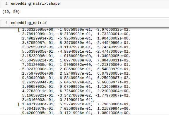
It’s a simple NumPy matrix where entry at index i is the pre-trained vector for the word of index i in our vectorizer’s vocabulary.

You can see that our embedding matrix has the shape of 19×50, because we had 19 unique words in our vocabulary and the GloVe pre-trained model file which we downloaded had 50-dimensional vectors.

You can play around with dimension, simply by changing the file or training your own model from scratch.

This embedding matrix can be used in any way you want. It can be fed into an embedding layer of a neural network, or just used for word similarity tasks.

And that’s GloVe, let’s move on to the next vectorization technique.

5. FastText

FastText was introduced by Facebook back in 2016. The idea behind FastText is very similar to Word2Vec. However, there was still one thing that methods like Word2Vec and GloVe lacked.

If you’ve been paying attention, you must have noticed one thing that Word2Vec and GloVe have in common — how we download a pre-trained model and perform a lookup operation to fetch the required word embeddings. Even though both of these models have been trained on billions of words, that still means our vocabulary is limited.

How does FastText improve over others?

FastText improved over other methods because of its capability of generalization to unknown words, which had been missing all along in the other methods.

How does it do that?

• Instead of using words to build word embeddings, FastText goes one level deeper, i.e. at the character level. The building blocks are letters instead of words.
• Word embeddings obtained via FastText aren’t obtained directly. They’re a combination of lower-level embeddings.
• Using characters instead of words has another advantage. Less data is needed for training, as a word becomes its own context in a way, resulting in much more information that can be extracted from a piece of text.

Now let’s take a look at how FastText utilizes sub-word information.

• Let’s say we have the word ‘reading’, character n-grams of length 3-6 would be generated for this word in the following manner:

• Angular brackets denote the beginning and the end.
• Since there can be a huge number of n-grams, hashing is used and instead of learning an embedding for each unique n-gram, we learn total B embeddings, where B denotes the bucket size. The original paper used a bucket size of 2 million.
• Via this hashing function, each character n-gram (say, ‘eadi’) is mapped to an integer between 1 to B, and that index has the corresponding embedding.
• Finally, the complete word embedding is obtained by averaging these constituent n-gram embeddings.
• Although this hashing approach results in collisions, it helps control the vocabulary size to a great extent.

The network used in FastText is similar to what we’ve seen in Word2Vec, just like there we can train the FastText in two modes – CBOW and skip-gram, thus we won’t be repeating that part here again. If you want to read more about Fasttext in detail, you can refer to the original papers here – paper-1 and paper-2.

Let’s move ahead and see what all things we can do with FastText.

You can install fasttext with pip.

pip install fasttext

You can either download a pre-trained fasttext model from here or you can train your own fasttext model and use it as a text classifier.

Since we have already seen enough of pre-trained models and it’s no different even in this case, so in this section, we’ll be focusing on how to create your own fasttext classifier.

Let’s say we have the following dataset, where there’s conversational text regarding a few drugs and we have to classify those texts into 3 types, i.e. with the kind of drugs with which they’re associated.

Now to train a fasttext classifier model on any dataset, we need to prepare the input data in a certain format which is:

__label__<label value><space><associated datapoint>

We’ll be doing this for our dataset too.

all_texts = train[‘text’].tolist() all_labels = train[‘drug type’].tolist() prep_datapoints=[] for i in range(len(all_texts)): sample = ‘__label__’+ str(all_labels[i]) + ‘ ‘+ all_texts[i] prep_datapoints.append(sample)

I omitted a lot of preprocessing in this step, in the real world it’s best to do rigorous preprocessing to make data fit for modeling.

Let’s write these prepared data points to a .txt file.

with open(‘train_fasttext.txt’,’w’) as f: for datapoint in prep_datapoints: f.write(datapoint) f.write(‘n’) f.close()

Now we have everything we need to train a fasttext model.

model = fasttext.train_supervised(‘train_fasttext.txt’)

Since our problem is a supervised classification problem, we trained a supervised Model.

Similarly, we can also obtain predictions from our trained model.

The model gives out the predicted label as well as the corresponding confidence score.

Again, the performance of this model depends on a lot of factors just like any other model, but if you want to have a quick peek at what the baseline accuracy should be, fasttext could be a very good choice.

So this was all about fasttext and how you can use it.

Wrapping up!

In this article we covered all the main branches of word embeddings, starting from naive count-based methods to sub-word level contextual embeddings. With the ever-rising utility of Natural Language Processing, it’s imperative that one is fully aware of its building blocks.

Given how much we read about the stuff which happens behind the curtains and the use cases of these methods, I hope now when you stumble across an NLP problem, you’ll be able to make an informed decision about which embedding technique to go with.

Future directions

I hope it goes without saying that whatever we covered in this article wasn’t exhaustive, and there are many more techniques out there to explore. These were just the main pillars.

Logically, the next step should be towards reading more about document (sentence) level embeddings, since we’ve covered the basics here. I would encourage you to read about things like Google’s BERT, Universal Sentence Encoder, and related topics.

If you decide to try BERT, start with this. It offers an amazing way to leverage BERT’s power without letting your machine do all the heavy lifting. Go through the README to get it set up.

That’s all for now. Thanks for reading!

Source: https://t-tees.com
Category: HOW