
The cube root function involves the cube root symbol ∛ (which stands for cube root) and hence let us recall a few things about it. The cube root of a number ‘a’ is a number ‘b’ such that b3 = a. i.e., if b3 = a ⇒ b = ∛a. i.e., if ‘b’ is the cube of ‘a’ then ‘a’ is the cube root of ‘b’. Some examples are:
- 23 = 8 ⇒ ∛8 = 2
- (-2)3 = -8 ⇒ ∛(-8) = -2
- 03 = 0 ⇒ ∛0 = 0
Thus, the cube root of a positive number is positive and that of a negative number is negative. Let us use all these facts to understand the cube root function.
You are viewing: Which Cube Root Function Is Always Decreasing As X Increases
1. What is Cube Root Function? 2. Domain and Range of Cube Root Function 3. Asymptotes of Cube Root Function 4. Graphing Parent Cube Root Function 5. Graphing Cube Root Functions 6. Properties of Cube Root Function 7. FAQs on Cube Root Function
The cube root function is the inverse of the cubic function. We know that the parent cubic function is of the form f(x) = x3 and this function is increasing, one-one, and onto. Hence, it is a bijection. Thus, its inverse function, which is cube root function, is of the form f(x) = ∛x is also a bijection. We know that a function and its inverse function are symmetric with respect to the line y = x and so the graphs of the parent cubic function and parent cube root functions look like this.

f(x) = ∛x is the basic/parent cube root function. But transformations may be applied on this function. Thus, the general form of cube root function is:
- f(x) = a ∛(bx – h) + k
Here, a, b, h, and k are real numbers where ‘h’ represents the horizontal translation, ‘k’ represents the vertical translation, and ‘a’ and ‘b’ represent the dilations.
We have already seen in the introduction that the cube root is defined for all numbers (positive, real, and 0). Thus, for any cube root function f(x), there is no x where f(x) is not defined. Thus, its domain is the set of all real numbers (R). In the same way, a cube root function results in all numbers (positive, real, and 0), and hence its range is also the set of all real numbers. Thus, a cube root function is f(x): R → R. i.e.,
- The domain of a cube root function is R.
- The range of a cube root function is R.
Read more : Which Hawaiian Island Is The Cheapest
The asymptotes of a function are lines where a part of the graph is very close to those lines but it actually doesn’t touch the lines. Let us take the parent cube root function f(x) = ∛x. Then
- As x → ±∞, f(x) → ±∞ and hence it doesn’t have horizontal asymptotes.
- There is no ‘x’ where f(x) is not defined and hence it doesn’t have vertical asymptotes.
Thus, a cube root function doesn’t have any asymptotes.
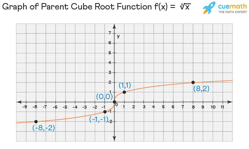
We have already seen that the domain and range of a cube root function is the set of all real numbers and it has no asymptotes. Let us see how to graph the parent cubic root function f(x) = ∛x first and later we will extend this process to graph any general cube root function. Let us construct a table of values with some random real numbers (as the domain is the set of all real numbers) for x (with some to be positive, some to be negative, and also a 0). Let us substitute each value in the function f(x) = ∛x to find the corresponding y-value.
x y -8 ∛(-8) = -2 -1 ∛(-1) = -1 0 ∛0 = 0 1 ∛1 = 1 8 ∛8 = 2
Here, we have chosen -8, -1, 0, 1, and 8 to be the x values as they are perfect cubes and they will help us to calculate y-values easily. Now, the points from the table are (-8, -2), (-1, -1), (0, 0), (1, 1), and (8, 2). Let us plot all these points on the graph sheet and join them by a curve which gives the graph of the cube root function f(x) = ∛x. Also, do not forget to extend the graph on both sides.
To graph any cube root function of the form, f(x) = a ∛(bx – h) + k, just take the same table as above and get new x and y-coordinates as follows according to the given function:
- To get new y-coordinates., apply the outside operations of the cube root sign on the y-coordinates of the above table.
- To get new x-coordinates, set bx – h equal to each of the old x-coordinates and solve for x that gives the new x-coordinates.
Here is an example.
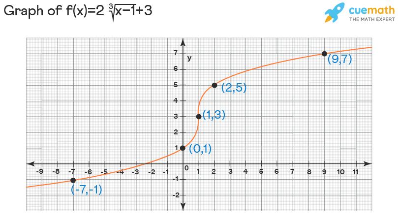
Example: Graph the cube root function f(x) = 2 ∛(x – 1) + 3.
Solution:
Let us consider the old table (of parent cube root function that is mentioned above).
x y -8 -2 -1 -1 0 0 1 1 8 2
Let us get the new table that will correspond to the given function in the following manner.
- The new x-coordinates can be obtained by setting x – 1 = old coordinate and solving for x.
- The new y-coordinates can be obtained by simplifying 2(old y-coordinate) + 3.
x y x – 1 = -8 ⇒ x = -7 2(-2) + 3 = -1 x – 1 = -1 ⇒ x = 0 2(-1) + 3 = 1 x – 1 = 0 ⇒ x = 1 2(0) + 3 = 3 x – 1 = 1 ⇒ x = 2 2(1) + 3 = 5 x – 1 = 8 ⇒ x = 9 2(2) + 3 = 7
The points from the table are (-7, -1), (0, 1), (1, 3), (2, 5), and (9, 7). Let us plot them, join them by a curve, and extend the curve.
Here are the characteristics of a cube root function f(x) = ∛x. We can look at the graph of the parent cube root function to justify each of the following properties.
- It is increasing on (-∞, ∞).
- It is positive on (0, ∞) and negative on (-∞, 0). f(x) = 0 when x = 0.
- Thus, the end behavior of the cube root function is: f(x) → ∞ as x → ∞ f(x) → -∞ as x → -∞
- It has no relative max/min.
- It has no global max/min.
- It has no asymptotes.
- Its domain and range is equal to (-∞, ∞).
☛ Related Topics:
- Cube Root Formula
- Cube Root Calculator
- Cube Root 1 to 20
- Square Root Formula
Source: https://t-tees.com
Category: WHICH